New Fermi Surveys

We’re pleased to be able to provide a new set of Fermi surveys. Fermi is the highest energy survey in SkyView and heretofore we had been providing two bands of Fermi data, from 100 to 5450 MHz and 5450 MHz to 300 GeV. Fermi’s resolution is a very strong function of energy. With the bands we’d originally chosen, low energy, low resolution photons blurred the images of most sources. While the top band had very reasonable resolution, it had relatively few photons. The new Fermi data is broken into 5 bands:

  1. 30-100 MeV
  2. 100-300 MeV
  3. 300-1000 MeV
  4. 1-3 GeV
  5. 3-300 GeV

This seems to give a cleaner separation of the low energy/resolution data while keeping enough photons in the higher energy bands to really show the sky. This all sky image shows data from bands 3-5.

Fermi RGB all sky image

RGB image using Fermi bands 3, 4 and 5. Click for high res version

Harder gamma-ray sources show as blue. A myriad Galactic and high-latitude sources show.

We’ve imaginatively named these surveys Fermi 1, 2, 3, 4 and 5 in order of increasing energy. They contain all of the Fermi data available through the beginning of April 2012. The Fermi sky exposure is now considered to be sufficiently uniform that we are providing these surveys as counts maps rather than intensity maps. We’ll be adding exposure information soon.

Posted in Documentation, Notices | Tagged , | 4 Comments

WISE All-Sky Data Available in SkyView

SkyView is now serving the data from the WISE All-Sky Data release. The main difference with the preliminary release is coverage on the ~40% of the sky that was missing in the earlier release. However the entire dataset has been reprocessed using updated calibrations and such.

We download WISE data from IRSA in large tiles, caching each tile so that we never have to download the same tile twice. It can take a while for WISE images to be generated if there has been no request in that region before, even when you are requesting only a very small region. It can easily take a minute or more to get the files we need to generate your image. As our cache grows you’ll be more likely to hit it and access should be much faster. Once data are in the cache it takes only a couple of seconds to generate a typical image.

The WISE data give us a view of the infrared sky comparable to the DSS optical images in the optical. We anticipate WISE being one of SkyView’s most popular surveys.

Posted in Announce | Tagged , | 6 Comments

SkyView Surveys Summary: I

Recently we’ve been updating and systematizing some of the metadata we have on SkyView surveys, trying to make sure that we have consistent, quantitative description of each one. Some of the key metadata are the resolution of the survey on the sky, sensitivity and sky coverage. It’s quite difficult to provide single numbers for these in a consistent way. E.g., for lots of surveys the resolution varies depending upon where you are. In some cases it even depends upon the spectrum of the source.

So take this with a grain (or maybe even a spoonful) of salt, but here’s a graph of the nominal resolution of SkyView’s surveys as a function of wavelength.

The resolution of SkyView surveys as a function of frequency

Resolution of Surveys Available in SkyView


The surveys span about 18 orders of magnitude in frequency. That’s pretty amazing. If you want to get a sense of how big that range is, consider the ratio of the distance to the nearest stars to your height… An immense difference — but only 1% of the range of SkyView‘s frequency coverage!

Looking at the graph we can split surveys into three categories based on their resolution: High resolution surveys have better than 10″ resolution. Most of these are concentrated near the optical, but there are a couple of outliers. Medium resolution surveys, with resolutions of about 1’ are the most common. These surveys have resolution comparable to our eyes. A fair number of surveys have resolutions of a degree or more. This doesn’t necessarily mean they are less valuable. Sometimes you want to look at the forest and not the trees.

Posted in Discussion | 1 Comment

What are people interested in? (2)

A few years ago we posted an image of the sky which showed what people have been looking at. Here’s an update giving the distribution of pixel centers for the last 10,000,000 or so SkyView images (about the last 18 months). This doesn’t include images in Cartesian, TOAST, CobeCube or Aitoff projections, nor do we include data using Ecliptic coordinates. However these only account for about 0.5% of the images we generate, so they wouldn’t make much difference.
Density distribution for skyview images.
The image is an Aitoff projection in equatorial coordinates with a Galactic coordinate grid overlaid. The data were originally sampled into a Cartesian grid with 1 degree pixels and that was resampled into an Aitoff grid using the clip resampler.

The image is very different from what we saw a couple of years ago where there where lots of ‘tire tread’ patterns in the data as people retrieved data in very specific regions. This looks like it’s a fairer realization of what parts of the sky are interesting.

And what was the very top location? It’s not 0,0 — which is what I would have guessed — nor the Galactic center or pole. All of those have pretty high values too. But the single highest pixel count (with about 40,000 images generated) was for the pixel that includes the center of M31. A clear winner for the most popular object in the sky!

Posted in Discussion | Tagged | 3 Comments

WISE versus IRAS

Just to see the incredible improvement WISE makes over the IRAS data here are two images of the same region (0.2×0.2 degrees at RA=2h 40m, Dec=20). The IRAS image (from the IRIS 12 micron survey) is very pixelated… There’s almost nothing there.
IRAS 12 micron image (IRIS 12 survey)

The WISE 12 micron data shows vastly more detail. Even in this boring region dozens of objects are clearly detected.
WISE 12 micron image

Note that the WISE surveys have been set to use the loglog scaling by default. Many features will not show up using the log scaling that is the default for most surveys.

Posted in Discussion | Tagged , , , | 2 Comments

SkyView links to WISE Preliminary Release Data

Data from the Wide-field Infrared Survey Explorer (WISE) Preliminary Release are now available in SkyView. WISE has made 4 all-sky surveys at 3.4, 4.6, 12 and 22 microns. The WISE surveys provide a remarkable picture of the sky in the infrared.

The two longest WISE wavelengths correspond closely to the two shorter IRAS bands but WISE has vastly higher resolution and sensitivity. The two shorter WISE wavelengths fill in the gap between the 2MASS K band (2.16 microns) and the 12 micron data.

The preliminary release covers a bit over half the sky as shown in this coverage map from the WISE archive at IPAC.WISE Preliminary Release coverage

Note that WISE data are distributed in large chunks. When SkyView first observes a region it will download the WISE data from the IPAC archive which may take a while. Subsequent images from the same region should run much faster.

As the title of the survey suggests, a full WISE release is forthcoming and should be available next month. We’ll switch over to that as soon as it’s available through the appropriate VO protocols.

Posted in Announce, Notices | Tagged , | 2 Comments

Short downtime

SkyView was unavailable for a couple of hours this morning due to hardware maintenance. We mistakenly thought that it would not affect the site so we did not give any advanced warning. We apologize for that and the inconvenience.

Posted in Notices | Leave a comment

How big is the universe?

Sometimes we can get a sense of the immensity of the universe from mundane things. The odometer on my 10 year old car is approaching 186,000 miles. That’s about as far as light goes in a single second. It takes light about 1.5 seconds to go from the Earth to the Moon, so I haven’t even gone as far as the nearest celestial body. The solar system is small potatoes though. To get to the very nearest objects that someone using SkyView is likely to want to look at, it takes light over 4 years, over 120 million seconds. That’s a billion years of driving. I don’t think the warranty will hold out!

Posted in Discussion | Tagged | 4 Comments

Features in the Gallery: Don’t look too close.

We recently had a query about features in the image
.
You can see it in the Gallery.

There images seems to have a very sharp but colorful transition between the bottom left and top right, but there are also a series of red steps on the left. If you look very closely you may see the the white block has two steps parallel to (and of the same width) as the red steps.

What’s going on here?

There are several different things happening here. Almost everything we’re seeing is an artifact of how we chose to sample the data. If you look at the characteristics of the image in the link above, you’ll see that it’s only about 0.0272 degrees on a side. However the survey it is based on, the H-alpha composite image says that the pixels in the underlying data are 2.5′. That’s about 0.042 degrees. So the image we’re looking at covers less than a single pixel in the input data does. We’re immensely oversampled.

Once we realize this, it’s pretty clear that we’re seeing two pixels. The original data in in galactic coordinates, so the border between the two pixels is oblique rather than horizontal or vertical.

The colored stripe is a consequence of using the clip resampling and a rather large smoothing radius (11 in this case). This tends to blur the sharp edges between the pixels so that instead of seeing a step function at the edge between the two pixels, we see a gradual transition with a width of about a dozen pixels. A Stern Special color table means makes the transition look like a rainbow rather than a sequence of grays. The fact that the transitions seems to cover the entire color table is not meaningful. No matter how little dynamic range there is in the image, the default is to try to emphasize details by using the entire color table. In fact the two pixels are not especially different compared to other pixels in the image.

For me, the really hard thing to understand were the steps in the image. Where do they come from? To understand them you really need to understand the clip resampling that this image uses. We call the sampler clip resampling because the way it works is to superpose the grid of user defined pixels on top of the grid of survey pixels. The clip sampler assumes that the flux in each input pixel is evenly distributed over the pixels. In this case the output pixels are much smaller than the input pixels (by a factor of about 600) so they would form a dense almost rectilinear grid over the much coarser survey pixels. The key is the ‘almost’. We’re dealing with projections in the sky, so there are small distortions from rectilinearity. Some of the output pixels are a little bigger than others — and they tend to get larger as we move from right to left in the image. Larger pixels collect a little more flux and so the pixels get smoothing increasing values as we moved from right to left. However, the color table only has a few values that are available in the range of fluxes, so we get the step function that initially seems some mysterious.

If we’d used the Clip (Intensive) sampler, instead of the Clip (Flux conserving) the steps would disappear. This sampler divides each output pixel by the size of the output pixel so that it exactly cancels out the changes in pixel values.

skyview image clip intensive sampler

H-Alpha Comp image using Clip (Intensive) sampler

If we’d used the default nearest neighbor method, we’d also not have seen the steps.

On the other hand if we’d used the bi-linear interpolation or the higher order resamplers which try to smoothly interpolated between pixels, then the image will look entirely different since the gradient of the image in both directions will affect the image, not just the two pixels we happen to overlap.

H-Alpha Comp image using Nearest Neighbor sampler

The take home lesson here is that you shouldn’t oversample survey data too much — and you certainly don’t want to ascribe any meaning to features that are smaller than the survey resolution.

Posted in Discussion | Tagged , , | Leave a comment