Posts Tagged ‘Clip sampler’

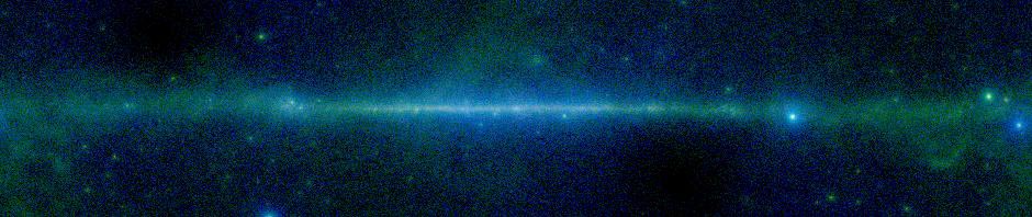
Features in the Gallery: Don’t look too close.

Monday, November 14th, 2011

We recently had a query about features in the image
.
You can see it in the Gallery.

There images seems to have a very sharp but colorful transition between the bottom left and top right, but there are also a series of red steps on the left. If you look very closely you may see the the white block has two steps parallel to (and of the same width) as the red steps.

What’s going on here?

There are several different things happening here. Almost everything we’re seeing is an artifact of how we chose to sample the data. If you look at the characteristics of the image in the link above, you’ll see that it’s only about 0.0272 degrees on a side. However the survey it is based on, the H-alpha composite image says that the pixels in the underlying data are 2.5′. That’s about 0.042 degrees. So the image we’re looking at covers less than a single pixel in the input data does. We’re immensely oversampled.

Once we realize this, it’s pretty clear that we’re seeing two pixels. The original data in in galactic coordinates, so the border between the two pixels is oblique rather than horizontal or vertical.

The colored stripe is a consequence of using the clip resampling and a rather large smoothing radius (11 in this case). This tends to blur the sharp edges between the pixels so that instead of seeing a step function at the edge between the two pixels, we see a gradual transition with a width of about a dozen pixels. A Stern Special color table means makes the transition look like a rainbow rather than a sequence of grays. The fact that the transitions seems to cover the entire color table is not meaningful. No matter how little dynamic range there is in the image, the default is to try to emphasize details by using the entire color table. In fact the two pixels are not especially different compared to other pixels in the image.

For me, the really hard thing to understand were the steps in the image. Where do they come from? To understand them you really need to understand the clip resampling that this image uses. We call the sampler clip resampling because the way it works is to superpose the grid of user defined pixels on top of the grid of survey pixels. The clip sampler assumes that the flux in each input pixel is evenly distributed over the pixels. In this case the output pixels are much smaller than the input pixels (by a factor of about 600) so they would form a dense almost rectilinear grid over the much coarser survey pixels. The key is the ‘almost’. We’re dealing with projections in the sky, so there are small distortions from rectilinearity. Some of the output pixels are a little bigger than others — and they tend to get larger as we move from right to left in the image. Larger pixels collect a little more flux and so the pixels get smoothing increasing values as we moved from right to left. However, the color table only has a few values that are available in the range of fluxes, so we get the step function that initially seems some mysterious.

If we’d used the Clip (Intensive) sampler, instead of the Clip (Flux conserving) the steps would disappear. This sampler divides each output pixel by the size of the output pixel so that it exactly cancels out the changes in pixel values.

skyview image clip intensive sampler

H-Alpha Comp image using Clip (Intensive) sampler

If we’d used the default nearest neighbor method, we’d also not have seen the steps.

On the other hand if we’d used the bi-linear interpolation or the higher order resamplers which try to smoothly interpolated between pixels, then the image will look entirely different since the gradient of the image in both directions will affect the image, not just the two pixels we happen to overlap.

H-Alpha Comp image using Nearest Neighbor sampler

The take home lesson here is that you shouldn’t oversample survey data too much — and you certainly don’t want to ascribe any meaning to features that are smaller than the survey resolution.

SkyView Version 2.6

Tuesday, December 15th, 2009

Version 2.6 of SkyView has been released. The major change is largely invisible to the users. When using the Clip sampler on large images we sometimes run into a problem where the corners of a user pixel when transformed into the survey projection, straddle a cut in the image. E.g., if the survey is an all-sky Cartesian projection, a user pixel crossing Longitude=180 may have corners to the far right and left of the survey image.

A new set of classes deals with straddles in Aitoff, Cartesian, TOAST and TEA projections. An update for the CSC projection should be available soon. Straddles are not an issue in projections like the Tangent plane (gnomonic) projection where there are no cuts in the image. The previous code could incorrectly sample data along the projection cuts.

Version 2.6 allows multiple values for the scaling keyword so that different surveys can be scaled differently. This can be especially useful for RGB imags.

A facility for allowing lower resolution images to be used when a user requests very large regions has been added to help support new optical surveys. This may be the first step in the direction of supporting hierarchical resolution images, a la, Google Sky and WWT.

The offset command used when drawing over an image has been enhanced.  By default offsets are made starting at the center of the image.  Instead of specifying two numeric values for the offset, an offset string of  “++”, “+-”, “-+”, or “–” may be given to offset to one of the corners of the image where the first character refers to the X-axis and the second to the Y-axis.  Offsets are added together so, e.g., to put draw text 100 pixels above and to the left of the lower right hand corner we could use the commands

   offset +-
   text -100 100 0 MyText

or

   offset +-
   offset -100 100
   text 0 0 0 MyText